Digital Twin of a TCSI System

Table of Contents

1. Introduction
2. Modelling The Engine
3. Fault Scenarios
4. Residuals Generation
5. Simulation Environment
6. Download

Introduction

Research on fault diagnosis and fault isolation on highly nonlinear dynamic systems such as the engine of a vehicle has garnered huge interest in recent years, especially with the automotive industry heading towards autonomous operations and big data. This digital twin (simulation testbed) of a single turbocharged petrol engine engine system is designed and developed for testing and evaluation of residuals generation and fault diagnosis methods.

This simulation testbed will serve as an excellent platform to demonstrate the effectiveness in simulating and presenting results on the fault diagnostic of automotive systems for the development and comparison of current and future research methods as well as for teaching initiatives. The engine model used is based on the mean value engine model (MVEM) with a PI-based boost controller. The simulation testbed is programmed in the Matlab/Simulink environment and it provides realistic simulations of the engine system with a selection of faults of interest and industrial-standard driving cycles via a GUI interface. The simulation kit is available free and as an open-source, and distributed under the GNU license.

If you use this simulation testbed in your research, please cite the following publication:

• K. Y. Ng, E. Frisk, M. Krysander, and L. Eriksson (2020), A Realistic Simulation Testbed of A Turbocharged Spark Ignited Engine System: A Platform for the Evaluation of Fault Diagnosis Algorithms and Strategies, IEEE Control Systems Magazine, vol. 40, no. 2, pp. 56–83. DOI:10.1109/MCS.2019.2961793.

Modelling The Engine

The simulation environment uses a 1.8L 4-cylinder single turbocharged spark ignited (TCSI) petrol engine as the testbed. It consists of the following subsystems; Air filter, Compressor, Intercooler, Throttle, Intake manifold, Engine block, Exhaust manifold, Turbine, Wastegate, and Exhaust system. The engine system is modelled using dynamical equations that describe the air flow through the subsystems in the engine. These equations are derived based on the mean value engine model (MVEM) for a single turbocharged petrol engine as reported by Eriksson in the following paper:

• L. Eriksson (2007), Modeling and control of turbocharged SI and DI engines, Oil & Gas Science and Technology-Revue de l’IFP, 62(4), pp. 523-538.

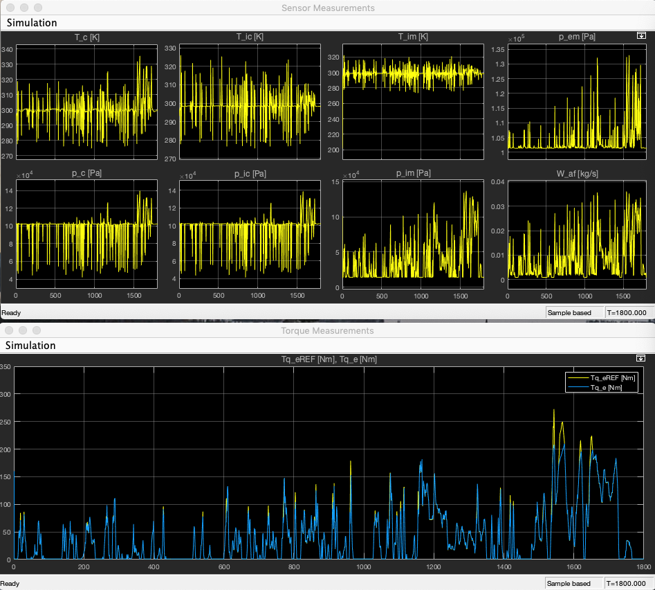
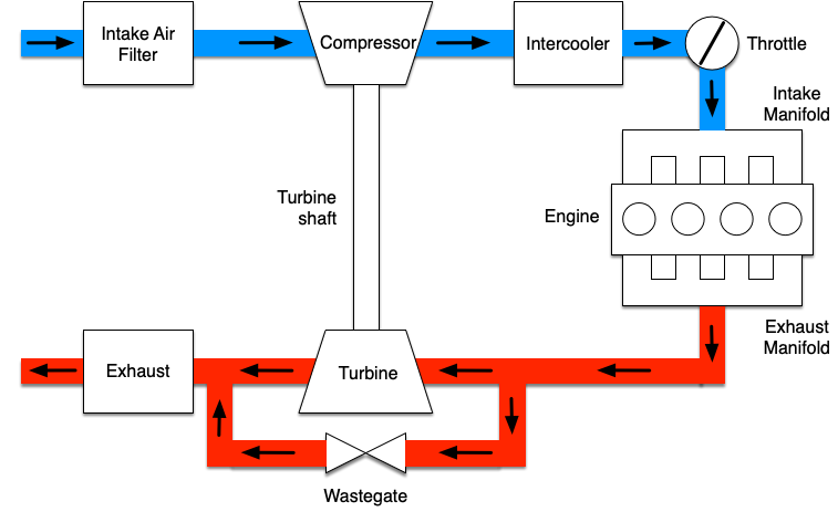A PI-based boost controller with anti-windup is used to produce the control inputs; Throttle effective area and Wastegate actuator for the turbocharger. In addition to the control inputs, the engine has the following actuators; Reference engine speed, Air-fuel ratio, Ambient pressure, and Ambient temperature. In addition, the engine has the following sensor measurements; Temperatures (compressor, intercooler, intake manifold), Pressures (compressor, intercooler, intake manifold, exhaust manifold), Air filter mass flow, and Engine torque.

The new European standard Worldwide harmonised Light vehicle Test Procedure (WLTP) driving cycle is used to verify the performance of the boost controller.

Fault Scenarios

The simulation testbed considers sensor, actuator, and variable faults in different parts of the engine system. There are 11 faults; 6 variable faults (fp_af, fC_vol, fW_af, fW_th, fW_c, fW_ic), 1 actuator measurement fault (fx_th), and 4 sensor measurement faults (fyW_af, fyp_im, fyp_ic, fyT_ic).

The faults are of different degrees of severity. Some faults are less severe and the engine can be reconfigured to a reduced performance operation mode to accommodate the faults until the vehicle is sent into the workshop for repair and maintenance. Some other faults are more severe that if not detected and isolated promptly, might cause permanent and serious damages to the engine system, which in turn will endanger the occupants in the vehicle as well as other road users.

Residuals Generation

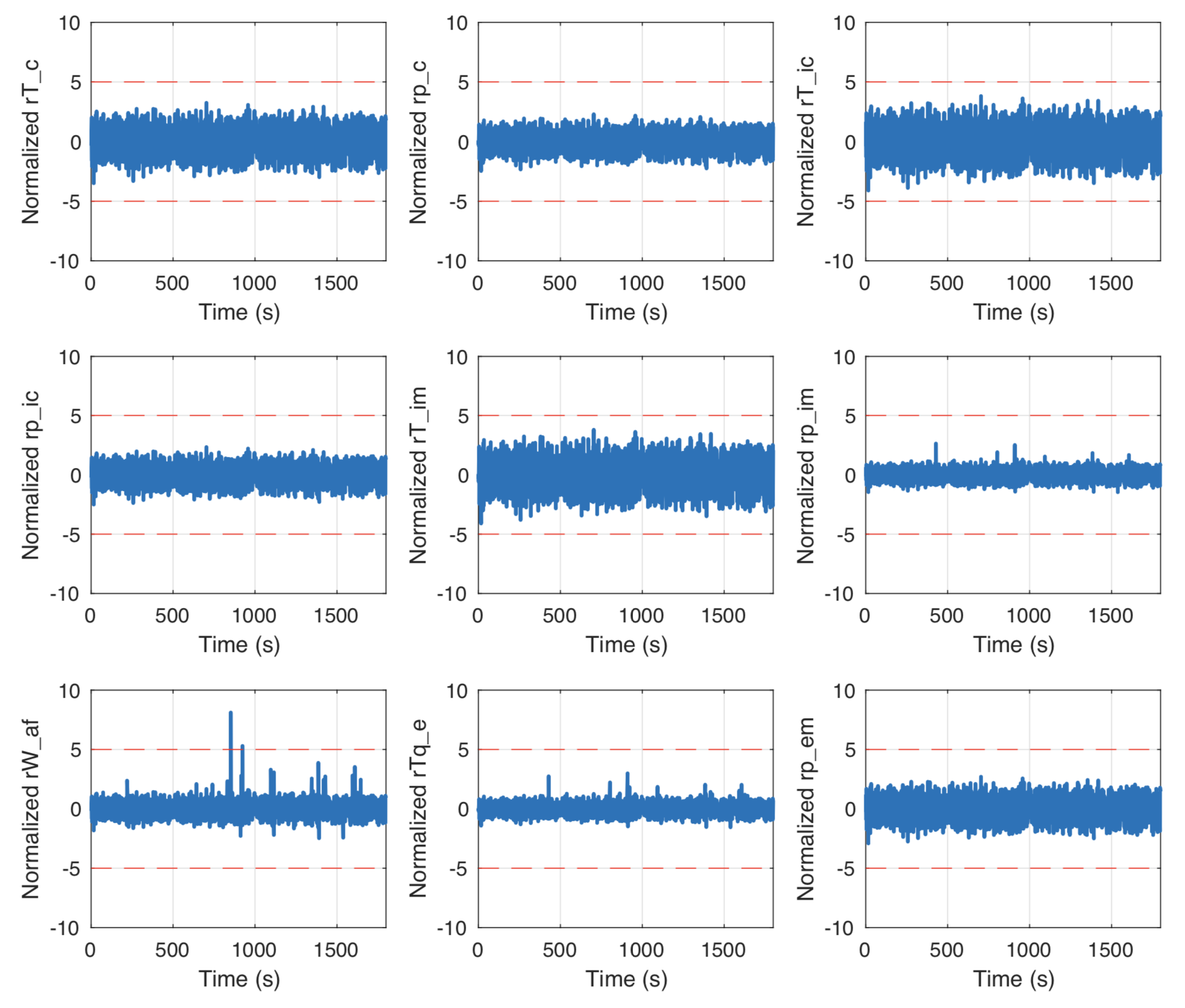
Initially, 9 residuals are generated based on the sensors setup of the engine system. These residuals are called the ‘Original 9’; rT_c, rp_c, rT_ic, rp_ic, rT_im, rp_im, rW_af, rTq_e, and rp_em. The residuals are generated by computing the difference between the sensor outputs of the model and the estimated outputs of an estimator/observer of the engine system: r_i = \hat y_i − y_i.

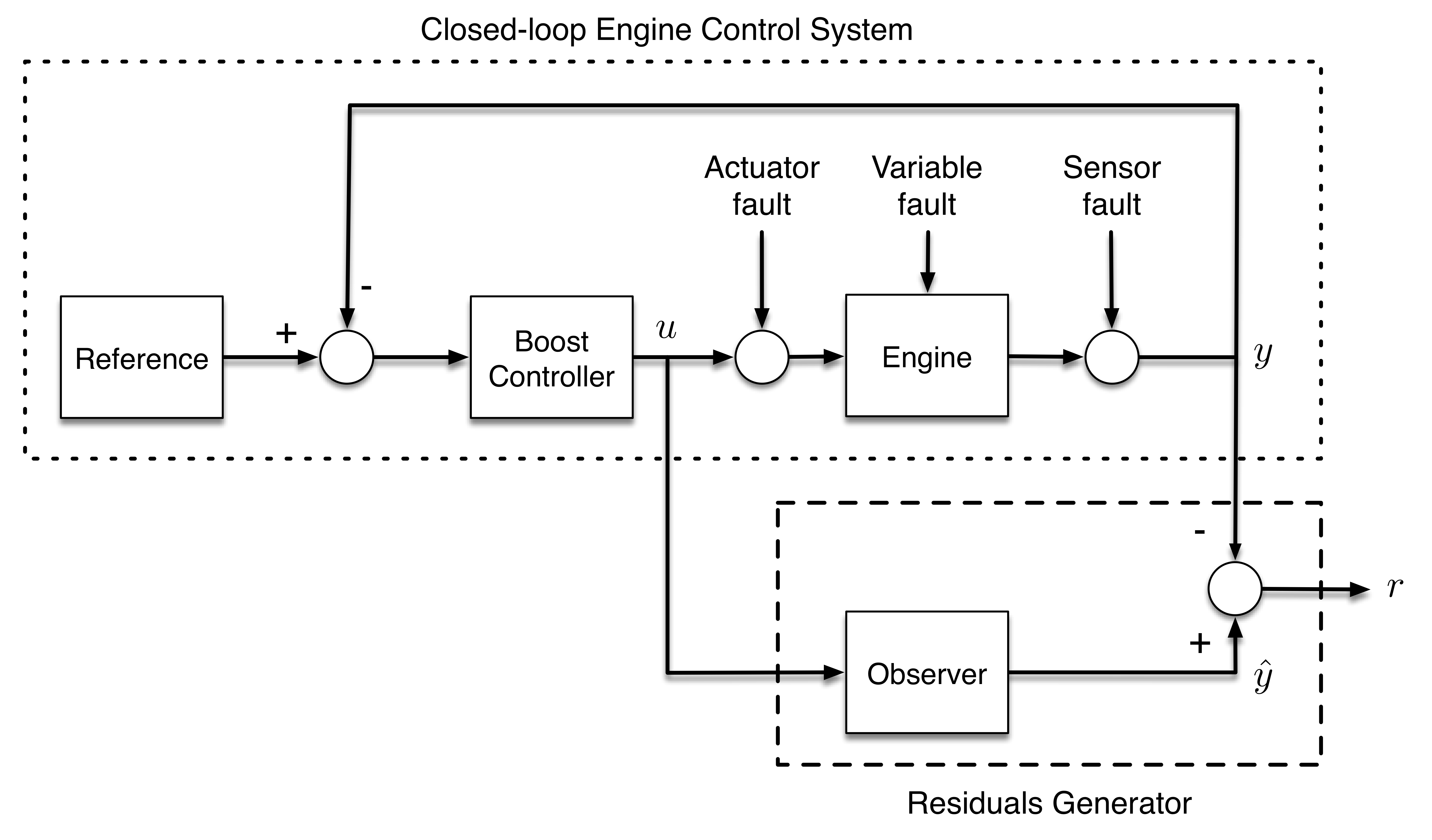
In a nominal fault-free scenario, all residuals have zero mean values.. This indicates that both the estimator and the model of the engine produce similar estimated and actual outputs, respectively, whilst being excited by the same control inputs. The default fault detection threshold, J = 5 determines if the residuals have triggered, i.e. |r_i| > J and hence, indicates that a fault has been detected. The value of the threshold, J, can be easily changed according to the designer’s wish. Conversely, in the presence of a fault, residuals that are sensitive to the corresponding faults would trigger and produce non-zero mean values.

 

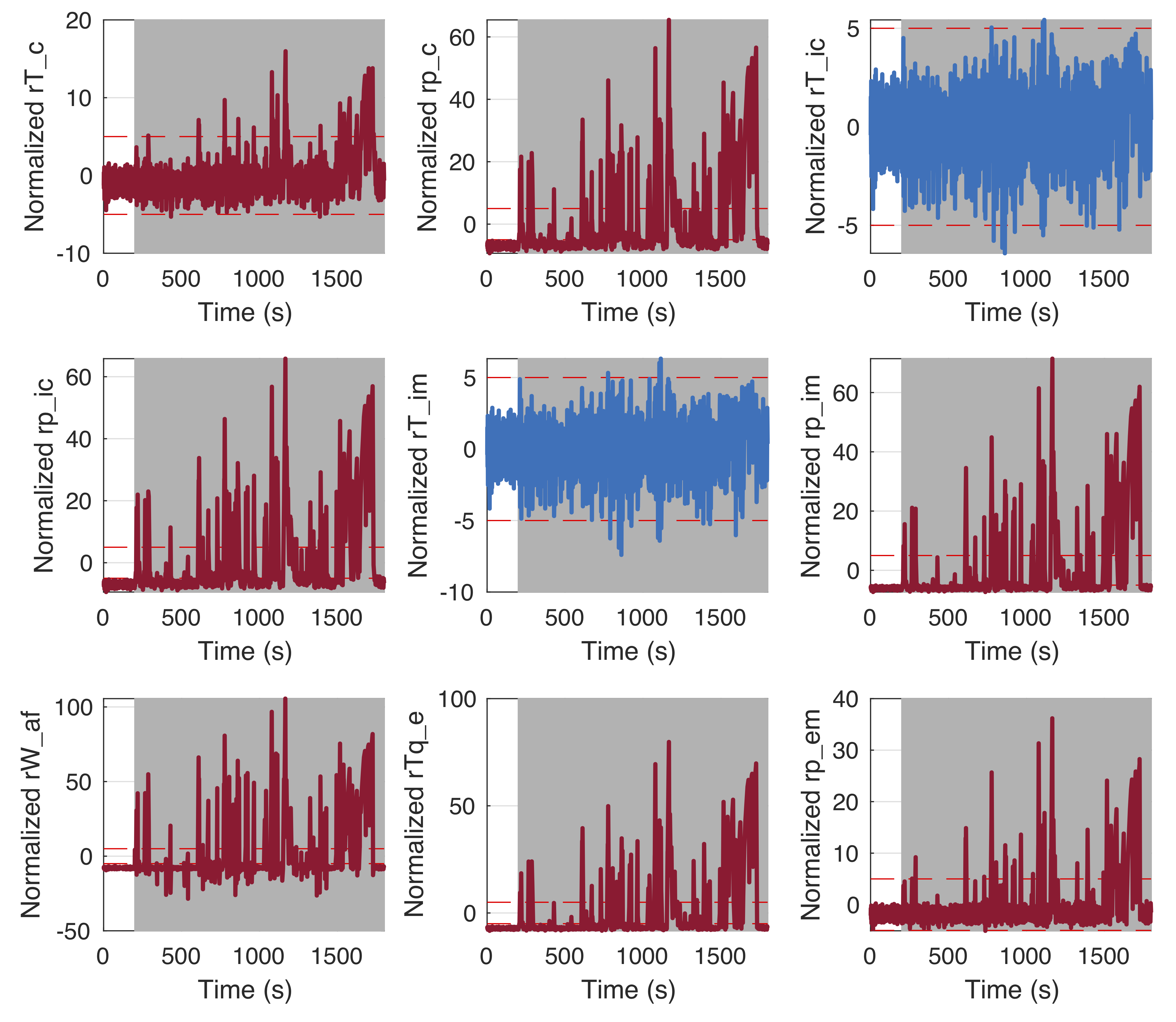
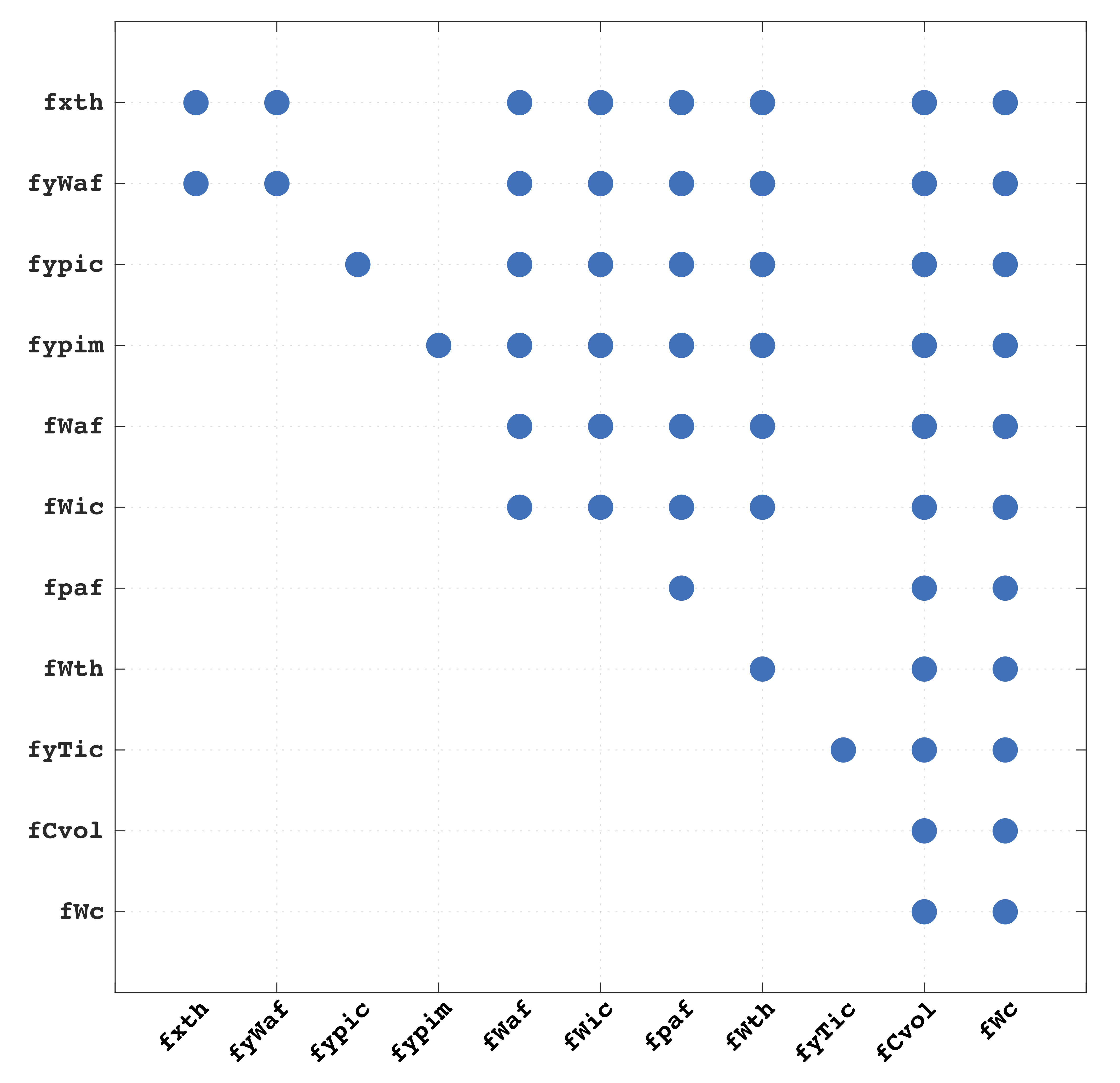By collectively identifying which residuals have triggered for the faults induced, fault isolation analysis to locate the fault in the engine system can then be performed. From the simulations for all faults, the Fault Sensitivity Matrix (FSM) is constructed. Using the FSM, the Fault Isolation Matrix (FIM) of the system for the current residuals design can then be generated. Therefore, this simulation testbed would serve as an excellent platform for designers and researchers to design and to perform Model-In-The-Loop tests of fault diagnosis schemes with application to actual automotive engine systems.

 
 
 

The Simulation Environment

The figure below shows the GUI of the simulation testbed in Matlab. Through this interface, the user can set the preferences for simulation settings, design and test their residuals generation and fault diagnosis schemes, as well as view simulation results. Do note that it will take some time to open and load the engine model during the initial runtime of Simulink for every new Matlab session.

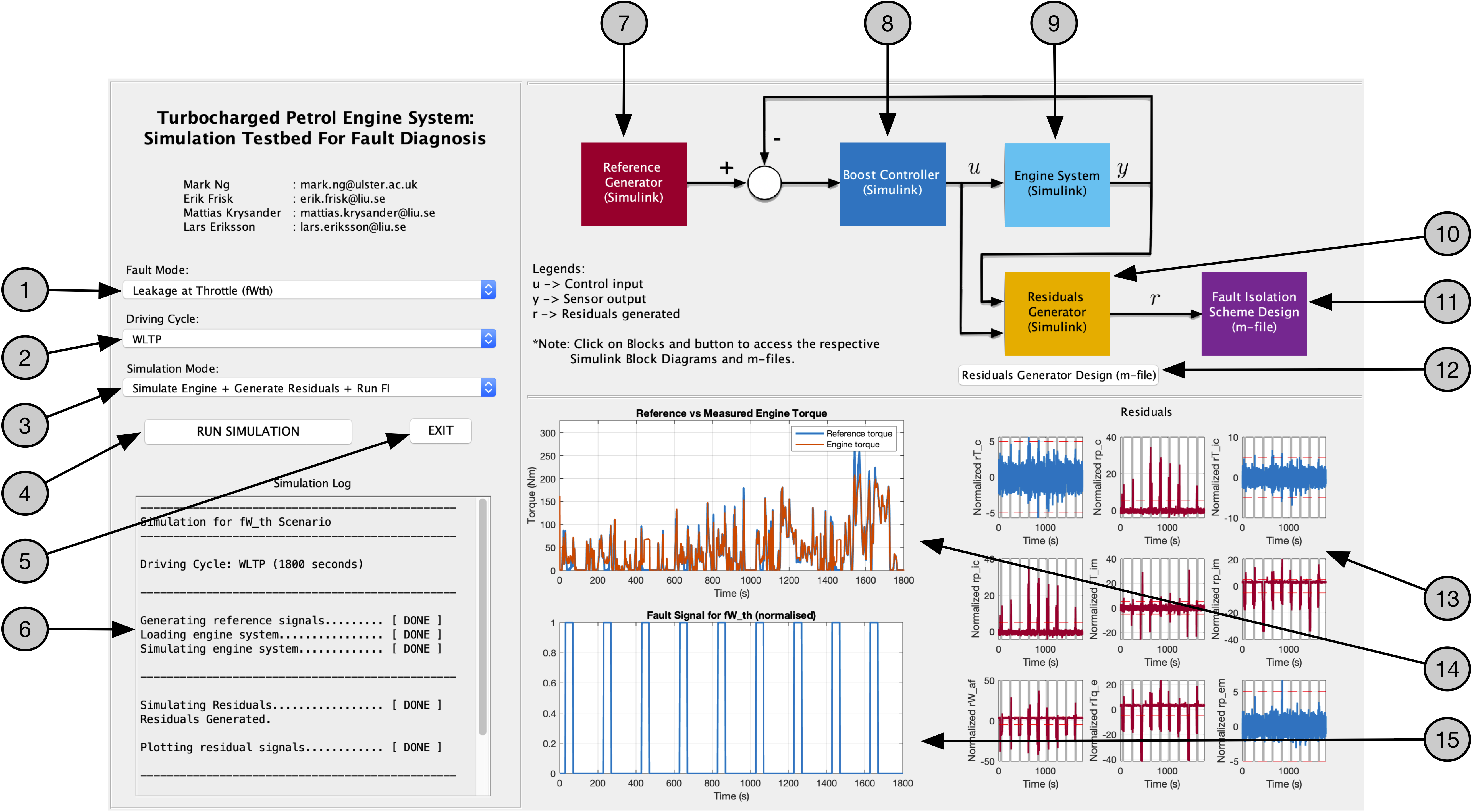
The main GUI of the simulation testbed in Matlab; 1) Sets the fault mode for simulation. 2) Sets the driving cycle. 3) Sets the simulation mode. 4) Runs the simulation. 5) Exits and closes the GUI. 6) Shows the simulation progress and log. 7) Click to open the reference generator Simulink model. 8–9) Click to open the boost controller and engine Simulink model. 10) Click to open the residuals generator Simulink model. 11) Click to open the fault diagnosis design scheme m-file. 12) Click to open the residuals generator design scheme m-file. 13) Displays the residuals generated. 14) Displays the reference torque vs actual torque of the engine. 15) Displays the fault signal induced (normalised).

 

On the left section of the GUI are popup menus for the user to establish some key simulation settings. The simulation settings available are as follows:

• Fault Mode: To induce any of the 11 faults available. A fault-free scenario is also available and is selected by default. As of current development, only single fault scenarios are available.
• Driving Cycle: A selection of 4 industrial standard driving cycles:
  • Worldwide harmonised Light vehicles Test Procedure (WLTP)
  • New European Driving Cycle (NEDC)
  • Extra-Urban Driving Cycle (EUDC)
  • EPA Federal Test Procedure (FTP-75)
• Simulation Mode: A choice of 2 simulation modes:
  • Simulate the engine only for the chosen driving cycle
  • Simulate the engine for the chosen driving cycle, generate the residuals, and run the fault diagnosis algorithm (the latter two functions would require design and coding inputs from the user)

On the top right section of the GUI, a block diagram representation of the engine control system, residuals generator, and fault diagnosis scheme can be found. The user can click on each block to access the corresponding Simulink model or m-file. For example, the user could use the ‘Residuals Generator (Simulink)’, ‘Residuals Generator Design (m-file)’, and ‘Fault Isolation Scheme Design (m-file)’ components to edit their design and codes for the residuals generation and fault diagnosis algorithms. The ‘RUN SIMULATION’ pushbutton starts the simulation and the ‘EXIT’ pushbutton exits the simulation environment and closes the GUI.

The results obtained from the simulation are displayed in the bottom right section of the GUI. The results displayed are the reference vs actual engine torque, and the normalised plot of the fault induced. A ‘Simulation Log’ is also available in the bottom left section of the GUI to show a summary of the simulation settings and to provide an update in real-time on the progress of the simulation. The plots and the ‘Simulation Log’ are automatically saved into the folder ‘/Results/DrivingCycle_FaultMode_Date’ that is located in the same directory as the simulation environment. A Matlab MAT-file containing key variables and data from the simulation is also saved.

The simulation kit contains the following key files:

• main.m - Main execution file. Run this file to start the GUI.
• Engine.mdl - Simulink model of the closed-loop nonlinear engine system. Open the model from the GUI using either the ‘Boost Controller (Simulink)’ or ‘Engine System (Simulink)’ blocks.
• GenerateResiduals.m - Codes for the residuals generation algorithm to be placed here. Open the file from the GUI using the ‘Residuals Generator Design (m-file)’ button.
• ResidualsGen.mdl - Simulink model of the residuals generator. The model is called and run from GenerateResiduals.m. The default residuals generated are also filtered and normalised, and added with signal noise. Open the model from the GUI using the ‘Residuals Generator (Simulink)’ block. Replace the ‘Residuals Generator’ in the Simulink model as desired to accommodate other methods for residuals generation.
• RunFI.m - Algorithm for fault diagnosis to be placed here. Open the file from the GUI using the ‘Fault Isolation Scheme Design (m-file)’ block.

Simulation Outputs and Saved Data

• omega_eREF_sync - reference engine speed
• Tq_eREF_sync - reference engine torque
• inputSig_sync - 5 actuator measurements to the engine (control inputs for throttle position area and wastegate, engine speed, ambient temperature and pressure)
• outputSig_sync - 9 sensor measurements from the engine (temperatures for the compressor, intercooler, and intake manifold, pressures for the compressor, intercooler, intake manifold, and exhaust manifold), air filter mass flow, and engine torque)
• statesSig_sync - 13 states of the engine system (temperatures and pressures for the air filter, compressor, intercooler, intake manifold, exhaust manifold, and turbine, and the turbine speed)
• faultSig_sync - normalised data of the faults (the selected induced fault would have non-zero data, except when ‘Fault-free’ scenario is selected where all faults would have data of value zero)
• residualSig_sync - data for all ‘Original 9’ residuals based on the current sensors setup (rT_c, rp_c, rT_ic, rp_ic, rT_im, rp_im, rW_af, rTq_e, rp_em). Note that these data would only be generated if Simulation Mode 2 is selected.

Download

The simulation testbed can be downloaded here.

Acknowledgement

We would like to thank former engineering undergraduates from Monash University Malaysia; Chun Yik Ang, Marcus Jun Yi Lim, and Ricky Sutopo, and William McMillan from Ulster University for participating in the alpha- and beta-testing of the simulation testbed on various operating systems and providing feedback to help improve this model.